Archive for the ‘Docker’ Category
Integrate security aspects in a DevOps process
A diagram of a common DevOps lifecycle:
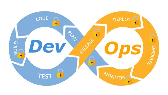
The DevOps world meant to provide complementary solution for both quick development (such as Agile) and a solution for cloud environments, where IT personnel become integral part of the development process. In the DevOps world, managing large number of development environments manually is practically infeasible. Monitoring mixed environments become a complex solution and deploying large number of different builds is becoming extremely fast and sensitive to changes.
The idea behind any DevOps solution is to provide a solution for deploying an entire CI/CD process, which means supporting constant changes and immediate deployment of builds/versions.
For the security department, this kind of process is at first look a nightmare – dozen builds, partial tests, no human control for any change, etc.
For this reason, it is crucial for the security department to embrace DevOps attitude, which means, embedding security in any part of the development lifecycle, software deployment or environment change.
It is important to understand that there are no constant stages as we used to have in waterfall development lifecycle, and most of the stages are parallel – in the CI/CD world everything changes quickly, components can be part of different stages, and for this reason it is important to confer the processes, methods and tools in all developments and DevOps teams.
In-order to better understand how to embed security into the DevOps lifecycle, we need to review the different stages in the development lifecycle:
Planning phase
This stage in the development process is about gathering business requirements.
At this stage, it is important to embed the following aspects:
- Gather information security requirements (such as authentication, authorization, auditing, encryptions, etc.)
- Conduct threat modeling in-order to detect possible code weaknesses
- Training / awareness programs for developers and DevOps personnel about secure coding
Creation / Code writing phase
This stage in the development process is about the code writing itself.
At this stage, it is important to embed the following aspects:
- Connect the development environments (IDE) to a static code analysis products
- Review the solution architecture by a security expert or a security champion on his behalf
- Review open source components embedded inside the code
Verification / Testing phase
This stage in the development process is about testing, conducted mostly by QA personnel.
At this stage, it is important to embed the following aspects:
- Run SAST (Static application security tools) on the code itself (pre-compiled stage)
- Run DAST (Dynamic application security tools) on the binary code (post-compile stage)
- Run IAST (Interactive application security tools) against the application itself
- Run SCA (Software composition analysis) tools in-order to detect known vulnerabilities in open source components or 3rd party components
Software packaging and pre-production phase
This stage in the development process is about software packaging of the developed code before deployment/distribution phase.
At this stage, it is important to embed the following aspects:
- Run IAST (Interactive application security tools) against the application itself
- Run fuzzing tools in-order to detect buffer overflow vulnerabilities – this can be done automatically as part of the build environment by embedding security tests for functional testing / negative testing
- Perform code signing to detect future changes (such as malwares)
Software packaging release phase
This stage is between the packaging and deployment stages.
At this stage, it is important to embed the following aspects:
- Compare code signature with the original signature from the software packaging stage
- Conduct integrity checks to the software package
- Deploy the software package to a development environment and conduct automate or stress tests
- Deploy the software package in a green/blue methodology for software quality and further security quality tests
Software deployment phase
At this stage, the software package (such as mobile application code, docker container, etc.) is moving to the deployment stage.
At this stage, it is important to embed the following aspects:
- Review permissions on destination folder (in case of code deployment for web servers)
- Review permissions for Docker registry
- Review permissions for further services in a cloud environment (such as storage, database, application, etc.) and fine-tune the service role for running the code
Configure / operate / Tune phase
At this stage, the development is in the production phase and passes modifications (according to business requirements) and on-going maintenance.
At this stage, it is important to embed the following aspects:
- Patch management processes or configuration management processes using tools such as Chef, Ansible, etc.
- Scanning process for detecting vulnerabilities using vulnerability assessment tools
- Deleting and re-deployment of vulnerable environments with an up-to-date environments (if possible)
On-going monitoring phase
At this stage, constant application monitoring is being conducted by the infrastructure or monitoring teams.
At this stage, it is important to embed the following aspects:
- Run RASP (Runtime application self-production) tools
- Implement defense at the application layer using WAF (Web application firewall) products
- Implement products for defending the application from Botnet attacks
- Implement products for defending the application from DoS / DDoS attacks
- Conduct penetration testing
- Implement monitoring solution using automated rules such as automated recovery of sensitive changes (tools such as GuardRails)
Security recommendations for developments based on CI/CD / DevOps process
- It is highly recommended to perform on-going training for the development and DevOps teams on security aspects and secure development
- It is highly recommended to nominate a security champion among the development and DevOps teams in-order to allow them to conduct threat modeling at early stages of the development lifecycle and in-order to embed security aspects as soon as possible in the development lifecycle
- Use automated tools for deploying environments in a simple and standard form.
Tools such as Puppet require root privileges for folders it has access to. In-order to lower the risk, it is recommended to enable folder access auditing. - Avoid storing passwords and access keys, hard-coded inside scripts and code.
- It is highly recommended to store credentials (SSH keys, privileged credentials, API keys, etc.) in a vault (Solutions such as HashiCorp vault or CyberArk).
- It is highly recommended to limit privilege access based on role (Role based access control) using least privileged.
- It is recommended to perform network separation between production environment and Dev/Test environments.
- Restrict all developer teams’ access to production environments, and allow only DevOps team’s access to production environments.
- Enable auditing and access control for all development environments and identify access attempts anomalies (such as developers access attempt to a production environment)
- Make sure sensitive data (such as customer data, credentials, etc.) doesn’t pass in clear text at transit. In-case there is a business requirement for passing sensitive data at transit, make sure the data is passed over encrypted protocols (such as SSH v2, TLS 1.2, etc.), while using strong cipher suites.
- It is recommended to follow OWASP organization recommendations (such as OWASP Top10, OWASP ASVS, etc.)
- When using Containers, it is recommended to use well-known and signed repositories.
- When using Containers, it is recommended not to rely on open source libraries inside the containers, and to conduct scanning to detect vulnerable versions (including dependencies) during the build creation process.
- When using Containers, it is recommended to perform hardening using guidelines such as CIS Docker Benchmark or CIS Kubernetes Benchmark.
- It is recommended to deploy automated tools for on-going tasks, starting from build deployments, code review for detecting vulnerabilities in the code and open source code, and patch management processes that will be embedded inside the development and build process.
- It is recommended to perform scanning to detect security weaknesses, using vulnerability management tools during the entire system lifetime.
- It is recommended to deploy configuration management tools, in-order to detect and automatically remediate configuration anomalies from the original configuration.
Additional reading sources:
- 20 Ways to Make Application Security Move at the Speed of DevOps
- The DevOps Security Checklist
- Making AppSec Testing Work in CI/CD
- Value driven threat modeling
- Automated Security Testing
- Security at the Speed of DevOps
- DevOps Security Best Practices
- The integration of DevOps and security
- When DevOps met Security - DevSecOps in a nutshell
- Grappling with DevOps Security
- Minimizing Risk and Improving Security in DevOps
- Security In A DevOps World
- Application Security in Devops
- Five Security Defenses Every Containerized Application Needs
- 5 ways to find and fix open source vulnerabilities
This article was written by Eyal Estrin, cloud security architect and Vitaly Unic, application security architect.
Separation Anxiety: A Tutorial for Isolating Your System with Linux Namespaces
With the advent of tools like Docker, Linux Containers, and others, it has become super easy to isolate Linux processes into their own little system environments. This makes it possible to run a whole range of applications on a single real Linux machine and ensure no two of them can interfere with each other, without having to resort to using virtual machines. These tools have been a huge boon to PaaS providers. But what exactly happens under the hood?
These tools rely on a number of features and components of the Linux kernel. Some of these features were introduced fairly recently, while others still require you to patch the kernel itself. But one of the key components, using Linux namespaces, has been a feature of Linux since version 2.6.24 was released in 2008.
Anyone familiar with chroot already has a basic idea of what Linux namespaces can do and how to use namespace generally. Just as chroot allows processes to see any arbitrary directory as the root of the system (independent of the rest of the processes), Linux namespaces allow other aspects of the operating system to be independently modified as well. This includes the process tree, networking interfaces, mount points, inter-process communication resources and more.
Why Use Namespaces for Process Isolation?
In a single-user computer, a single system environment may be fine. But on a server, where you want to run multiple services, it is essential to security and stability that the services are as isolated from each other as possible. Imagine a server running multiple services, one of which gets compromised by an intruder. In such a case, the intruder may be able to exploit that service and work his way to the other services, and may even be able compromise the entire server. Namespace isolation can provide a secure environment to eliminate this risk.
For example, using namespacing, it is possible to safely execute arbitrary or unknown programs on your server. Recently, there has been a growing number of programming contest and “hackathon” platforms, such as HackerRank, TopCoder, Codeforces, and many more. A lot of them utilize automated pipelines to run and validate programs that are submitted by the contestants. It is often impossible to know in advance the true nature of contestants’ programs, and some may even contain malicious elements. By running these programs namespaced in complete isolation from the rest of the system, the software can be tested and validated without putting the rest of the machine at risk. Similarly, online continuous integration services, such as Drone.io, automatically fetch your code repository and execute the test scripts on their own servers. Again, namespace isolation is what makes it possible to provide these services safely.
Namespacing tools like Docker also allow better control over processes’ use of system resources, making such tools extremely popular for use by PaaS providers. Services like Heroku and Google App Engine use such tools to isolate and run multiple web server applications on the same real hardware. These tools allow them to run each application (which may have been deployed by any of a number of different users) without worrying about one of them using too many system resources, or interfering and/or conflicting with other deployed services on the same machine. With such process isolation, it is even possible to have entirely different stacks of dependency softwares (and versions) for each isolated environment!
If you’ve used tools like Docker, you already know that these tools are capable of isolating processes in small “containers”. Running processes in Docker containers is like running them in virtual machines, only these containers are significantly lighter than virtual machines. A virtual machine typically emulates a hardware layer on top of your operating system, and then runs another operating system on top of that. This allows you to run processes inside a virtual machine, in complete isolation from your real operating system. But virtual machines are heavy! Docker containers, on the other hand, use some key features of your real operating system, including namespaces, and ensure a similar level of isolation, but without emulating the hardware and running yet another operating system on the same machine. This makes them very lightweight.
Process Namespace
Historically, the Linux kernel has maintained a single process tree. The tree contains a reference to every process currently running in a parent-child hierarchy. A process, given it has sufficient privileges and satisfies certain conditions, can inspect another process by attaching a tracer to it or may even be able to kill it.
With the introduction of Linux namespaces, it became possible to have multiple “nested” process trees. Each process tree can have an entirely isolated set of processes. This can ensure that processes belonging to one process tree cannot inspect or kill – in fact cannot even know of the existence of – processes in other sibling or parent process trees.
Every time a computer with Linux boots up, it starts with just one process, with process identifier (PID) 1. This process is the root of the process tree, and it initiates the rest of the system by performing the appropriate maintenance work and starting the correct daemons/services. All the other processes start below this process in the tree. The PID namespace allows one to spin off a new tree, with its own PID 1 process. The process that does this remains in the parent namespace, in the original tree, but makes the child the root of its own process tree.
With PID namespace isolation, processes in the child namespace have no way of knowing of the parent process’s existence. However, processes in the parent namespace have a complete view of processes in the child namespace, as if they were any other process in the parent namespace.
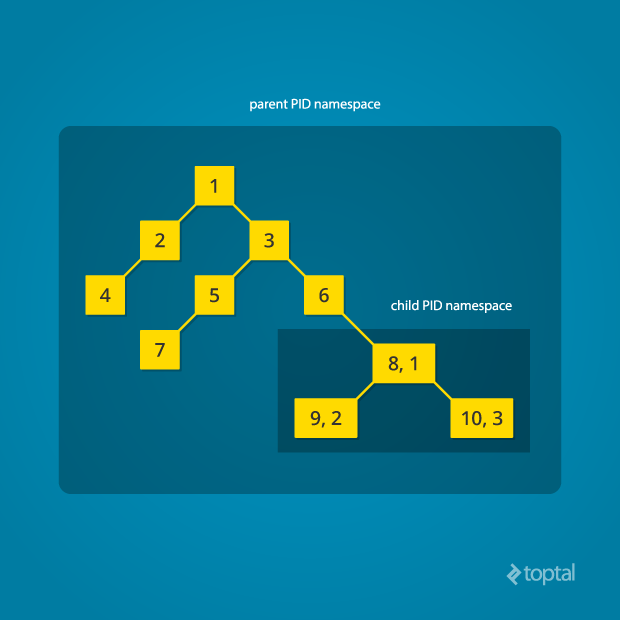
It is possible to create a nested set of child namespaces: one process starts a child process in a new PID namespace, and that child process spawns yet another process in a new PID namespace, and so on.
With the introduction of PID namespaces, a single process can now have multiple PIDs associated with it, one for each namespace it falls under. In the Linux source code, we can see that a struct named pid, which used to keep track of just a single PID, now tracks multiple PIDs through the use of a struct named upid:
struct upid {
  int nr;                     // the PID value
  struct pid_namespace *ns;   // namespace where this PID is relevant
  // ...
};

struct pid {
  // ...
  int level;                  // number of upids
  struct upid numbers[0];     // array of upids
};
To create a new PID namespace, one must call the clone() system call with a special flag CLONE_NEWPID. (C provides a wrapper to expose this system call, and so do many other popular languages.) Whereas the other namespaces discussed below can also be created using the unshare() system call, a PID namespace can only be created at the time a new process is spawned using clone(). Once clone() is called with this flag, the new process immediately starts in a new PID namespace, under a new process tree. This can be demonstrated with a simple C program:
#define _GNU_SOURCE
#include <sched.h>
#include <stdio.h>
#include <stdlib.h>
#include <sys/wait.h>
#include <unistd.h>

static char child_stack[1048576];

static int child_fn() {
  printf("PID: %ld\n", (long)getpid());
  return 0;
}

int main() {
  pid_t child_pid = clone(child_fn, child_stack+1048576, CLONE_NEWPID | SIGCHLD, NULL);
  printf("clone() = %ld\n", (long)child_pid);

  waitpid(child_pid, NULL, 0);
  return 0;
}
Compile and run this program with root privileges and you will notice an output that resembles this:
clone() = 5304
PID: 1
The PID, as printed from within the child_fn, will be 1.
Even though this namespace tutorial code above is not much longer than “Hello, world” in some languages, a lot has happened behind the scenes. The clone() function, as you would expect, has created a new process by cloning the current one and started execution at the beginning of the child_fn() function. However, while doing so, it detached the new process from the original process tree and created a separate process tree for the new process.
Try replacing the static int child_fn() function with the following, to print the parent PID from the isolated process’s perspective:
static int child_fn() {
  printf("Parent PID: %ld\n", (long)getppid());
  return 0;
}
Running the program this time yields the following output:
clone() = 11449
Parent PID: 0
Notice how the parent PID from the isolated process’s perspective is 0, indicating no parent. Try running the same program again, but this time, remove the CLONE_NEWPID flag from within the clone() function call:
pid_t child_pid = clone(child_fn, child_stack+1048576, SIGCHLD, NULL);
This time, you will notice that the parent PID is no longer 0:
clone() = 11561
Parent PID: 11560
However, this is just the first step in our tutorial. These processes still have unrestricted access to other common or shared resources. For example, the networking interface: if the child process created above were to listen on port 80, it would prevent every other process on the system from being able to listen on it.
Linux Network Namespace
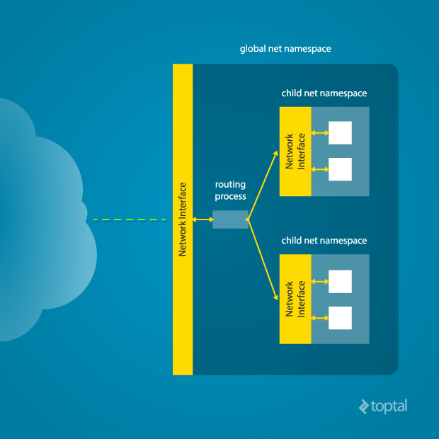
This is where a network namespace becomes useful. A network namespace allows each of these processes to see an entirely different set of networking interfaces. Even the loopback interface is different for each network namespace.
Isolating a process into its own network namespace involves introducing another flag to the clone() function call: CLONE_NEWNET;
#define _GNU_SOURCE
#include <sched.h>
#include <stdio.h>
#include <stdlib.h>
#include <sys/wait.h>
#include <unistd.h>


static char child_stack[1048576];

static int child_fn() {
  printf("New `net` Namespace:\n");
  system("ip link");
  printf("\n\n");
  return 0;
}

int main() {
  printf("Original `net` Namespace:\n");
  system("ip link");
  printf("\n\n");

  pid_t child_pid = clone(child_fn, child_stack+1048576, CLONE_NEWPID | CLONE_NEWNET | SIGCHLD, NULL);

  waitpid(child_pid, NULL, 0);
  return 0;
}
Output:
Original `net` Namespace:
1: lo: <LOOPBACK,UP,LOWER_UP> mtu 65536 qdisc noqueue state UNKNOWN mode DEFAULT group default
    link/loopback 00:00:00:00:00:00 brd 00:00:00:00:00:00
2: enp4s0: <BROADCAST,MULTICAST,UP,LOWER_UP> mtu 1500 qdisc pfifo_fast state UP mode DEFAULT group default qlen 1000
    link/ether 00:24:8c:a1:ac:e7 brd ff:ff:ff:ff:ff:ff


New `net` Namespace:
1: lo: <LOOPBACK> mtu 65536 qdisc noop state DOWN mode DEFAULT group default
    link/loopback 00:00:00:00:00:00 brd 00:00:00:00:00:00
What’s going on here? The physical ethernet device enp4s0 belongs to the global network namespace, as indicated by the “ip” tool run from this namespace. However, the physical interface is not available in the new network namespace. Moreover, the loopback device is active in the original network namespace, but is “down” in the child network namespace.
In order to provide a usable network interface in the child namespace, it is necessary to set up additional “virtual” network interfaces which span multiple namespaces. Once that is done, it is then possible to create Ethernet bridges, and even route packets between the namespaces. Finally, to make the whole thing work, a “routing process” must be running in the global network namespace to receive traffic from the physical interface, and route it through the appropriate virtual interfaces to to the correct child network namespaces. Maybe you can see why tools like Docker, which do all this heavy lifting for you, are so popular!
To do this by hand, you can create a pair of virtual Ethernet connections between a parent and a child namespace by running a single command from the parent namespace:
ip link add name veth0 type veth peer name veth1 netns <pid>
Here, <pid> should be replaced by the process ID of the process in the child namespace as observed by the parent. Running this command establishes a pipe-like connection between these two namespaces. The parent namespace retains the veth0 device, and passes the veth1 device to the child namespace. Anything that enters one of the ends, comes out through the other end, just as you would expect from a real Ethernet connection between two real nodes. Accordingly, both sides of this virtual Ethernet connection must be assigned IP addresses.
Mount Namespace
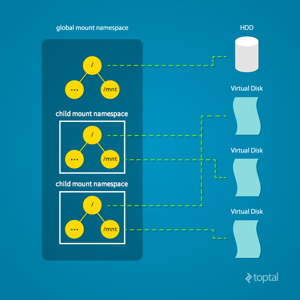
Linux also maintains a data structure for all the mountpoints of the system. It includes information like what disk partitions are mounted, where they are mounted, whether they are readonly, et cetera. With Linux namespaces, one can have this data structure cloned, so that processes under different namespaces can change the mountpoints without affecting each other.
Creating separate mount namespace has an effect similar to doing a chroot(). chroot() is good, but it does not provide complete isolation, and its effects are restricted to the root mountpoint only. Creating a separate mount namespace allows each of these isolated processes to have a completely different view of the entire system’s mountpoint structure from the original one. This allows you to have a different root for each isolated process, as well as other mountpoints that are specific to those processes. Used with care per this tutorial, you can avoid exposing any information about the underlying system.
The clone() flag required to achieve this is CLONE_NEWNS:
clone(child_fn, child_stack+1048576, CLONE_NEWPID | CLONE_NEWNET | CLONE_NEWNS | SIGCHLD, NULL)
Initially, the child process sees the exact same mountpoints as its parent process would. However, being under a new mount namespace, the child process can mount or unmount whatever endpoints it wants to, and the change will affect neither its parent’s namespace, nor any other mount namespace in the entire system. For example, if the parent process has a particular disk partition mounted at root, the isolated process will see the exact same disk partition mounted at the root in the beginning. But the benefit of isolating the mount namespace is apparent when the isolated process tries to change the root partition to something else, as the change will only affect the isolated mount namespace.
Interestingly, this actually makes it a bad idea to spawn the target child process directly with the CLONE_NEWNS flag. A better approach is to start a special “init” process with the CLONE_NEWNS flag, have that “init” process change the “/”, “/proc”, “/dev” or other mountpoints as desired, and then start the target process. This is discussed in a little more detail near the end of this namespace tutorial.
Other Namespaces
There are other namespaces that these processes can be isolated into, namely user, IPC, and UTS. The user namespace allows a process to have root privileges within the namespace, without giving it that access to processes outside of the namespace. Isolating a process by the IPC namespace gives it its own interprocess communication resources, for example, System V IPC and POSIX messages. The UTS namespace isolates two specific identifiers of the system: nodename and domainname.
A quick example to show how UTS namespace is isolated is shown below:
#define _GNU_SOURCE
#include <sched.h>
#include <stdio.h>
#include <stdlib.h>
#include <sys/utsname.h>
#include <sys/wait.h>
#include <unistd.h>


static char child_stack[1048576];

static void print_nodename() {
  struct utsname utsname;
  uname(&utsname);
  printf("%s\n", utsname.nodename);
}

static int child_fn() {
  printf("New UTS namespace nodename: ");
  print_nodename();

  printf("Changing nodename inside new UTS namespace\n");
  sethostname("GLaDOS", 6);

  printf("New UTS namespace nodename: ");
  print_nodename();
  return 0;
}

int main() {
  printf("Original UTS namespace nodename: ");
  print_nodename();

  pid_t child_pid = clone(child_fn, child_stack+1048576, CLONE_NEWUTS | SIGCHLD, NULL);

  sleep(1);

  printf("Original UTS namespace nodename: ");
  print_nodename();

  waitpid(child_pid, NULL, 0);

  return 0;
}
This program yields the following output:
Original UTS namespace nodename: XT
New UTS namespace nodename: XT
Changing nodename inside new UTS namespace
New UTS namespace nodename: GLaDOS
Original UTS namespace nodename: XT
Here, child_fn() prints the nodename, changes it to something else, and prints it again. Naturally, the change happens only inside the new UTS namespace.
More information on what all of the namespaces provide and isolate can be found in the tutorial here
Cross-Namespace Communication
Often it is necessary to establish some sort of communication between the parent and the child namespace. This might be for doing configuration work within an isolated environment, or it can simply be to retain the ability to peek into the condition of that environment from outside. One way of doing that is to keep an SSH daemon running within that environment. You can have a separate SSH daemon inside each network namespace. However, having multiple SSH daemons running uses a lot of valuable resources like memory. This is where having a special “init” process proves to be a good idea again.
The “init” process can establish a communication channel between the parent namespace and the child namespace. This channel can be based on UNIX sockets or can even use TCP. To create a UNIX socket that spans two different mount namespaces, you need to first create the child process, then create the UNIX socket, and then isolate the child into a separate mount namespace. But how can we create the process first, and isolate it later? Linux provides unshare(). This special system call allows a process to isolate itself from the original namespace, instead of having the parent isolate the child in the first place. For example, the following code has the exact same effect as the code previously mentioned in the network namespace section:
#define _GNU_SOURCE
#include <sched.h>
#include <stdio.h>
#include <stdlib.h>
#include <sys/wait.h>
#include <unistd.h>


static char child_stack[1048576];

static int child_fn() {
  // calling unshare() from inside the init process lets you create a new namespace after a new process has been spawned
  unshare(CLONE_NEWNET);

  printf("New `net` Namespace:\n");
  system("ip link");
  printf("\n\n");
  return 0;
}

int main() {
  printf("Original `net` Namespace:\n");
  system("ip link");
  printf("\n\n");

  pid_t child_pid = clone(child_fn, child_stack+1048576, CLONE_NEWPID | SIGCHLD, NULL);

  waitpid(child_pid, NULL, 0);
  return 0;
}
And since the “init” process is something you have devised, you can make it do all the necessary work first, and then isolate itself from the rest of the system before executing the target child.
Conclusion
This tutorial is just an overview of how to use namespaces in Linux. It should give you a basic idea of how a Linux developer might start to implement system isolation, an integral part of the architecture of tools like Docker or Linux Containers. In most cases, it would be best to simply use one of these existing tools, which are already well-known and tested. But in some cases, it might make sense to have your very own, customized process isolation mechanism, and in that case, this namespace tutorial will help you out tremendously.
There is a lot more going on under the hood than I’ve covered in this article, and there are more ways you might want to limit your target processes for added safety and isolation. But, hopefully, this can serve as a useful starting point for someone who is interested in knowing more about how namespace isolation with Linux really works.
Originally from Toptal
Scaling Scala: How to Dockerize Using Kubernetes
Kubernetes is the new kid on the block, promising to help deploy applications into the cloud and scale them more quickly. Today, when developing for a microservices architecture, it’s pretty standard to choose Scala for creating API servers.
If there is a Scala application in your plans and you want to scale it into a cloud, then you are at the right place. In this article I am going to show step-by-step how to take a generic Scala application and implement Kubernetes with Docker to launch multiple instances of the application. The final result will be a single application deployed as multiple instances, and load balanced by Kubernetes.
All of this will be implemented by simply importing the Kubernetes source kit in your Scala application. Please note, the kit hides a lot of complicated details related to installation and configuration, but it is small enough to be readable and easy to understand if you want to analyze what it does. For simplicity, we will deploy everything on your local machine. However, the same configuration is suitable for a real-world cloud deployment of Kubernetes.

What is Kubernetes?
Before going into the gory details of the implementation, let’s discuss what Kubernetes is and why it’s important.
You may have already heard of Docker. In a sense, it is a lightweight virtual machine.
For these reasons, it is already one of the more widely used tools for deploying applications in clouds. A Docker image is pretty easy and fast to build and duplicable, much easier than a traditional virtual machine like VMWare, VirtualBox, or XEN.
Kubernetes complements Docker, offering a complete environment for managing dockerized applications. By using Kubernetes, you can easily deploy, configure, orchestrate, manage, and monitor hundreds or even thousands of Docker applications.
Kubernetes is an open source tool developed by Google and has been adopted by many other vendors. Kubernetes is available natively on the Google cloud platform, but other vendors have adopted it for their OpenShift cloud services too. It can be found on Amazon AWS, Microsoft Azure, RedHat OpenShift, and even more cloud technologies. We can say it is well positioned to become a standard for deploying cloud applications.
Prerequisites
Now that we covered the basics, let’s check if you have all the prerequisite software installed. First of all, you need Docker. If you are using either Windows or Mac, you need the Docker Toolbox. If you are using Linux, you need to install the particular package provided by your distribution or simply follow the official directions.
We are going to code in Scala, which is a JVM language. You need, of course, the Java Development Kit and the scala SBT tool installed and available in the global path. If you are already a Scala programmer, chances are you have those tools already installed.
If you are using Windows or Mac, Docker will by default create a virtual machine named default with only 1GB of memory, which can be too small for running Kubernetes. In my experience, I had issues with the default settings. I recommend that you open the VirtualBox GUI, select your virtual machine default, and change the memory to at least to 2048MB.

The Application to Clusterize
The instructions in this tutorial can apply to any Scala application or project. For this article to have some “meat” to work on, I chose an example used very often to demonstrate a simple REST microservice in Scala, called Akka HTTP. I recommend you try to apply source kit to the suggested example before attempting to use it on your application. I have tested the kit against the demo application, but I cannot guarantee that there will be no conflicts with your code.
So first, we start by cloning the demo application:
git clone https://github.com/theiterators/akka-http-microservice
Next, test if everything works correctly:
cd akka-http-microservice
sbt run
Then, access to http://localhost:9000/ip/8.8.8.8, and you should see something like in the following image:

Adding the Source Kit
Now, we can add the source kit with some Git magic:
git remote add ScalaGoodies https://github.com/sciabarra/ScalaGoodies
git fetch --all
git merge ScalaGoodies/kubernetes
With that, you have the demo including the source kit, and you are ready to try. Or you can even copy and paste the code from there into your application.
Once you have merged or copied the files in your projects, you are ready to start.
Starting Kubernetes
Once you have downloaded the kit, we need to download the necessary kubectl binary, by running:
bin/install.sh
This installer is smart enough (hopefully) to download the correct kubectl binary for OSX, Linux, or Windows, depending on your system. Note, the installer worked on the systems I own. Please do report any issues, so that I can fix the kit.
Once you have installed the kubectl binary, you can start the whole Kubernetes in your local Docker. Just run:
bin/start-local-kube.sh
The first time it is run, this command will download the images of the whole Kubernetes stack, and a local registry needed to store your images. It can take some time, so please be patient. Also note, it needs direct accesses to the internet. If you are behind a proxy, it will be a problem as the kit does not support proxies. To solve it, you have to configure the tools like Docker, curl, and so on to use the proxy. It is complicated enough that I recommend getting a temporary unrestricted access.
Assuming you were able to download everything successfully, to check if Kubernetes is running fine, you can type the following command:
bin/kubectl get nodes
The expected answer is:
NAME        STATUS    AGE
127.0.0.1   Ready     2m
Note that age may vary, of course. Also, since starting Kubernetes can take some time, you may have to invoke the command a couple of times before you see the answer. If you do not get errors here, congratulations, you have Kubernetes up and running on your local machine.
Dockerizing Your Scala App
Now that you have Kubernetes up and running, you can deploy your application in it. In the old days, before Docker, you had to deploy an entire server for running your application. With Kubernetes, all you need to do to deploy your application is:
- Create a Docker image.
- Push it in a registry from where it can be launched.
- Launch the instance with Kubernetes, that will take the image from the registry.
Luckily, it is way less complicated that it looks, especially if you are using the SBT build tool like many do.
In the kit, I included two files containing all the necessary definitions to create an image able to run Scala applications, or at least what is needed to run the Akka HTTP demo. I cannot guarantee that it will work with any other Scala applications, but it is a good starting point, and should work for many different configurations. The files to look for building the Docker image are:
docker.sbt
project/docker.sbt
Let’s have a look at what’s in them. The file project/docker.sbt contains the command to import the sbt-docker plugin:
addSbtPlugin("se.marcuslonnberg" % "sbt-docker" % "1.4.0")
This plugin manages the building of the Docker image with SBT for you. The Docker definition is in the docker.sbt file and looks like this:
imageNames in docker := Seq(ImageName("localhost:5000/akkahttp:latest"))

dockerfile in docker := {
  val jarFile: File = sbt.Keys.`package`.in(Compile, packageBin).value
  val classpath = (managedClasspath in Compile).value
  val mainclass = mainClass.in(Compile, packageBin).value.getOrElse(sys.error("Expected exactly one main class"))
  val jarTarget = s"/app/${jarFile.getName}"
  val classpathString = classpath.files.map("/app/" + _.getName)
    .mkString(":") + ":" + jarTarget
  new Dockerfile {
    from("anapsix/alpine-java:8")
    add(classpath.files, "/app/")
    add(jarFile, jarTarget)
    entryPoint("java", "-cp", classpathString, mainclass)
  }
}
To fully understand the meaning of this file, you need to know Docker well enough to understand this definition file. However, we are not going into the details of the Docker definition file, because you do not need to understand it thoroughly to build the image.
the SBT will take care of collecting all the files for you.
Note the classpath is automatically generated by the following command:
val classpath = (managedClasspath in Compile).value
In general, it is pretty complicated to gather all the JAR files to run an application. Using SBT, the Docker file will be generated with add(classpath.files, "/app/"). This way, SBT collects all the JAR files for you and constructs a Dockerfile to run your application.
The other commands gather the missing pieces to create a Docker image. The image will be built using an existing image APT to run Java programs (anapsix/alpine-java:8, available on the internet in the Docker Hub). Other instructions are adding the other files to run your application. Finally, by specifying an entry point, we can run it. Note also that the name starts with localhost:5000 on purpose, because localhost:5000 is where I installed the registry in the start-kube-local.sh script.
Building the Docker Image with SBT
To build the Docker image, you can ignore all the details of the Dockerfile. You just need to type:
sbt dockerBuildAndPush
The sbt-docker plugin will then build a Docker image for you, downloading from the internet all the necessary pieces, and then it will push to a Docker registry that was started before, together with the Kubernetes application in localhost. So, all you need is to wait a little bit more to have your image cooked and ready.
Note, if you experience problems, the best thing to do is to reset everything to a known state by running the following commands:
bin/stop-kube-local.sh
bin/start-kube-local.sh
Those commands should stop all the containers and restart them correctly to get your registry ready to receive the image built and pushed by sbt.
Starting the Service in Kubernetes
Now that the application is packaged in a container and pushed in a registry, we are ready to use it. Kubernetes uses the command line and configuration files to manage the cluster. Since command lines can become very long, and also be able to replicate the steps, I am using the configurations files here. All the samples in the source kit are in the folder kube.
Our next step is to launch a single instance of the image. A running image is called, in the Kubernetes language, a pod. So let’s create a pod by invoking the following command:
bin/kubectl create -f kube/akkahttp-pod.yml
You can now inspect the situation with the command:
bin/kubectl get pods
You should see:
NAME                   READY     STATUS    RESTARTS   AGE
akkahttp               1/1       Running   0          33s
k8s-etcd-127.0.0.1     1/1       Running   0          7d
k8s-master-127.0.0.1   4/4       Running   0          7d
k8s-proxy-127.0.0.1    1/1       Running   0          7d
Status actually can be different, for example, “ContainerCreating”, it can take a few seconds before it becomes “Running”. Also, you can get another status like “Error” if, for example, you forget to create the image before.
You can also check if your pod is running with the command:
bin/kubectl logs akkahttp
You should see an output ending with something like this:
[DEBUG] [05/30/2016 12:19:53.133] [default-akka.actor.default-dispatcher-5] [akka://default/system/IO-TCP/selectors/$a/0] Successfully bound to /0:0:0:0:0:0:0:0:9000
Now you have the service up and running inside the container. However, the service is not yet reachable. This behavior is part of the design of Kubernetes. Your pod is running, but you have to expose it explicitly. Otherwise, the service is meant to be internal.
Creating a Service
Creating a service and checking the result is a matter of executing:
bin/kubectl create -f kube/akkahttp-service.yaml
bin/kubectl get svc
You should see something like this:
NAME               CLUSTER-IP   EXTERNAL-IP   PORT(S)    AGE
akkahttp-service   10.0.0.54                  9000/TCP   44s
kubernetes         10.0.0.1     <none>        443/TCP    3m
Note that the port can be different. Kubernetes allocated a port for the service and started it. If you are using Linux, you can directly open the browser and type http://10.0.0.54:9000/ip/8.8.8.8 to see the result. If you are using Windows or Mac with Docker Toolbox, the IP is local to the virtual machine that is running Docker, and unfortunately it is still unreachable.
I want to stress here that this is not a problem of Kubernetes, rather it is a limitation of the Docker Toolbox, which in turn depends on the constraints imposed by virtual machines like VirtualBox, which act like a computer within another computer. To overcome this limitation, we need to create a tunnel. To make things easier, I included another script which opens a tunnel on an arbitrary port to reach any service we deployed. You can type the following command:
bin/forward-kube-local.sh akkahttp-service 9000
Note that the tunnel will not run in the background, you have to keep the terminal window open as long as you need it and close when you do not need the tunnel anymore. While the tunnel is running, you can open: http://localhost:9000/ip/8.8.8.8 and finally see the application running in Kubernetes.
Final Touch: Scale
So far we have “simply” put our application in Kubernetes. While it is an exciting achievement, it does not add too much value to our deployment. We’re saved from the effort of uploading and installing on a server and configuring a proxy server for it.
Where Kubernetes shines is in scaling. You can deploy two, ten, or one hundred instances of our application by only changing the number of replicas in the configuration file. So let’s do it.
We are going to stop the single pod and start a deployment instead. So let’s execute the following commands:
bin/kubectl delete -f kube/akkahttp-pod.yml
bin/kubectl create -f kube/akkahttp-deploy.yaml
Next, check the status. Again, you may try a couple of times because the deployment can take some time to be performed:
NAME                                   READY     STATUS    RESTARTS   AGE
akkahttp-deployment-4229989632-mjp6u   1/1       Running   0          16s
akkahttp-deployment-4229989632-s822x   1/1       Running   0          16s
k8s-etcd-127.0.0.1                     1/1       Running   0          6d
k8s-master-127.0.0.1                   4/4       Running   0          6d
k8s-proxy-127.0.0.1                    1/1       Running   0          6d
Now we have two pods, not one. This is because in the configuration file I provided, there is the value replica: 2, with two different names generated by the system. I am not going into the details of the configuration files, because the scope of the article is simply an introduction for Scala programmers to jump-start into Kubernetes.
Anyhow, there are now two pods active. What is interesting is that the service is the same as before. We configured the service to load balance between all the pods labeled akkahttp. This means we do not have to redeploy the service, but we can replace the single instance with a replicated one.
We can verify this by launching the proxy again (if you are on Windows and you have closed it):
bin/forward-kube-local.sh akkahttp-service 9000
Then, we can try to open two terminal windows and see the logs for each pod. For example, in the first type:
bin/kubectl logs -f akkahttp-deployment-4229989632-mjp6u
And in the second type:
bin/kubectl logs -f akkahttp-deployment-4229989632-s822x
Of course, edit the command line accordingly with the values you have in your system.
Now, try to access the service with two different browsers. You should expect to see the requests to be split between the multiple available servers, like in the following image:

Conclusion
Today we barely scratched the surface. Kubernetes offers a lot more possibilities, including automated scaling and restart, incremental deployments, and volumes. Furthermore, the application we used as an example is very simple, stateless with the various instances not needing to know each other. In the real world, distributed applications do need to know each other, and need to change configurations according to the availability of other servers. Indeed, Kubernetes offers a distributed keystore (etcd) to allow different applications to communicate with each other when new instances are deployed. However, this example is purposefully small enough and simplified to help you get going, focusing on the core functionalities. If you follow the tutorial, you should be able to get a working environment for your Scala application on your machine without being confused by a large number of details and getting lost in the complexity.
This article was written by Michele Sciabarra, a Toptal Scala developer.
Getting Started with Docker: Simplifying Devops
If you like whales, or are simply interested in quick and painless continuous delivery of your software to production, then I invite you to read this introductory Docker Tutorial. Everything seems to indicate that software containers are the future of IT, so let’s go for a quick dip with the container whales Moby Dock andMolly.

Docker, represented by a logo with a friendly looking whale, is an open source project that facilitates deployment of applications inside of software containers. Its basic functionality is enabled by resource isolation features of the Linux kernel, but it provides a user-friendly API on top of it. The first version was released in 2013, and it has since become extremely popular and is being widely used by many big players such as eBay, Spotify, Baidu, and more. In the last funding round, Docker has landed a huge $95 million.
Transporting Goods Analogy
The philosophy behind Docker could be illustrated with a following simple analogy. In the international transportation industry, goods have to be transported by different means like forklifts, trucks, trains, cranes, and ships. These goods come in different shapes and sizes and have different storing requirements: sacks of sugar, milk cans, plants etc. Historically, it was a painful process depending on manual intervention at every transit point for loading and unloading.

It has all changed with the uptake of intermodal containers. As they come in standard sizes and are manufactured with transportation in mind, all the relevant machineries can be designed to handle these with minimal human intervention. The additional benefit of sealed containers is that they can preserve the internal environment like temperature and humidity for sensitive goods. As a result, the transportation industry can stop worrying about the goods themselves and focus on getting them from A to B.

And here is where Docker comes in and brings similar benefits to the software industry.
How Is It Different from Virtual Machines?
At a quick glance, virtual machines and Docker containers may seem alike. However, their main differences will become apparent when you take a look at the following diagram:

Applications running in virtual machines, apart from the hypervisor, require a full instance of the operating system and any supporting libraries. Containers, on the other hand, share the operating system with the host. Hypervisor is comparable to the container engine (represented as Docker on the image) in a sense that it manages the lifecycle of the containers. The important difference is that the processes running inside the containers are just like the native processes on the host, and do not introduce any overheads associated with hypervisor execution. Additionally, applications can reuse the libraries and share the data between containers.
As both technologies have different strengths, it is common to find systems combining virtual machines and containers. A perfect example is a tool named Boot2Docker described in the Docker installation section.
Docker Architecture

At the top of the architecture diagram there are registries. By default, the main registry is the Docker Hub which hosts public and official images. Organizations can also host their private registries if they desire.
On the right-hand side we have images and containers. Images can be downloaded from registries explicitly (docker pull imageName) or implicitly when starting a container. Once the image is downloaded it is cached locally.
Containers are the instances of images – they are the living thing. There could be multiple containers running based on the same image.
At the centre, there is the Docker daemon responsible for creating, running, and monitoring containers. It also takes care of building and storing images. Finally, on the left-hand side there is a Docker client. It talks to the daemon via HTTP. Unix sockets are used when on the same machine, but remote management is possible via HTTP based API.
Installing Docker
For the latest instructions you should always refer to the official documentation.
Docker runs natively on Linux, so depending on the target distribution it could be as easy as sudo apt-get install docker.io. Refer to the documentation for details. Normally in Linux, you prepend the Docker commands with sudo, but we will skip it in this article for clarity.
As the Docker daemon uses Linux-specific kernel features, it isn’t possible to run Docker natively in Mac OS or Windows. Instead, you should install an application called Boot2Docker. The application consists of a VirtualBox Virtual Machine, Docker itself, and the Boot2Docker management utilities. You can follow the official installation instructions for MacOS and Windows to install Docker on these platforms.
Using Docker
Let us begin this section with a quick example:
docker run phusion/baseimage echo "Hello Moby Dock. Hello Molly."
We should see this output:
Hello Moby Dock. Hello Molly.
However, a lot more has happened behind the scenes than you may think:
- The image ‘phusion/baseimage’ was download from Docker Hub (if it wasn’t already in local cache)
- A container based on this image was started
- The command echo was executed within the container
- The container was stopped when the command exitted
On first run, you may notice a delay before the text is printed on screen. If the image had been cached locally, everything would have taken a fraction of a second. Details about the last container can be retrieved by by running docker ps -l:
CONTAINER ID		IMAGE					COMMAND				CREATED			STATUS				PORTS	NAMES
af14bec37930		phusion/baseimage:latest		"echo 'Hello Moby Do		2 minutes ago		Exited (0) 3 seconds ago		stoic_bardeen
Taking the Next Dive
As you can tell, running a simple command within Docker is as easy as running it directly on a standard terminal. To illustrate a more practical use case, throughout the remainder of this article, we will see how we can utilize Docker to deploy a simple web server application. To keep things simple, we will write a Java program that handles HTTP GET requests to ‘/ping’ and responds with the string ‘pong\n’.
import java.io.IOException;
import java.io.OutputStream;
import java.net.InetSocketAddress;
import com.sun.net.httpserver.HttpExchange;
import com.sun.net.httpserver.HttpHandler;
import com.sun.net.httpserver.HttpServer;

public class PingPong {

    public static void main(String[] args) throws Exception {
        HttpServer server = HttpServer.create(new InetSocketAddress(8080), 0);
        server.createContext("/ping", new MyHandler());
        server.setExecutor(null);
        server.start();
    }

    static class MyHandler implements HttpHandler {
        @Override
        public void handle(HttpExchange t) throws IOException {
            String response = "pong\n";
            t.sendResponseHeaders(200, response.length());
            OutputStream os = t.getResponseBody();
            os.write(response.getBytes());
            os.close();
        }
    }
}
Dockerfile
Before jumping in and building your own Docker image, it’s a good practice to first check if there is an existing one in the Docker Hub or any private registries you have access to. For example, instead of installing Java ourselves, we will use an official image: java:8.
To build an image, first we need to decide on a base image we are going to use. It is denoted by FROMinstruction. Here, it is an official image for Java 8 from the Docker Hub. We are going to copy it into our Java file by issuing a COPY instruction. Next, we are going to compile it with RUN. EXPOSE instruction denotes that the image will be providing a service on a particular port. ENTRYPOINT is an instruction that we want to execute when a container based on this image is started and CMD indicates the default parameters we are going to pass to it.
FROM java:8
COPY PingPong.java /
RUN javac PingPong.java
EXPOSE 8080
ENTRYPOINT ["java"]
CMD ["PingPong"]
After saving these instructions in a file called “Dockerfile”, we can build the corresponding Docker image by executing:
docker build -t toptal/pingpong .
The official documentation for Docker has a section dedicated to best practices regarding writing Dockerfile.
Running Containers
When the image has been built, we can bring it to life as a container. There are several ways we could run containers, but let’s start with a simple one:
docker run -d -p 8080:8080 toptal/pingpong
where -p [port-on-the-host]:[port-in-the-container] denotes the ports mapping on the host and the container respectively. Furthermore, we are telling Docker to run the container as a daemon process in the background by specifying -d. You can test if the web server application is running by attempting to access ‘http://localhost:8080/ping’. Note that on platforms where Boot2docker is being used, you will need to replace ‘localhost’ with the IP address of the virtual machine where Docker is running.
On Linux:
curl http://localhost:8080/ping
On platforms requiring Boot2Docker:
curl $(boot2docker ip):8080/ping
If all goes well, you should see the response:
pong
Hurray, our first custom Docker container is alive and swimming! We could also start the container in an interactive mode -i -t. In our case, we will override the entrypoint command so we are presented with a bash terminal. Now we can execute whatever commands we want, but exiting the container will stop it:
docker run -i -t --entrypoint="bash" toptal/pingpong
There are many more options available to use for starting up the containers. Let us cover a few more. For example, if we want to persist data outside of the container, we could share the host filesystem with the container by using -v. By default, the access mode is read-write, but could be changed to read-only mode by appending :ro to the intra-container volume path. Volumes are particularly important when we need to use any security information like credentials and private keys inside of the containers, which shouldn’t be stored on the image. Additionally, it could also prevent the duplication of data, for example by mapping your local Maven repository to the container to save you from downloading the Internet twice.
Docker also has the capability of linking containers together. Linked containers can talk to each other even if none of the ports are exposed. It can be achieved with –link other-container-name. Below is an example combining mentioned above parameters:
docker run -p 9999:8080
    --link otherContainerA --link otherContainerB
    -v /Users/$USER/.m2/repository:/home/user/.m2/repository
toptal/pingpongUnsurprisingly, the list of operations that one could apply to the containers and images is rather long. For brevity, let us look at just a few of them:
- stop – Stops a running container.
- start – Starts a stopped container.
- commit – Creates a new image from a container’s changes.
- rm – Removes one or more containers.
- rmi – Removes one or more images.
- ps – Lists containers.
- images – Lists images.
- exec – Runs a command in a running container.
Last command could be particularly useful for debugging purposes, as it lets you to connect to a terminal of a running container:
docker exec -i -t <container-id> bash
Docker Compose for the Microservice World
If you have more than just a couple of interconnected containers, it makes sense to use a tool like docker-compose. In a configuration file, you describe how to start the containers and how they should be linked with each other. Irrespective of the amount of containers involved and their dependencies, you could have all of them up and running with one command: docker-compose up.
Docker in the Wild
Let’s look at three stages of project lifecycle and see how our friendly whale could be of help.
Development
Docker helps you keep your local development environment clean. Instead of having multiple versions of different services installed such as Java, Kafka, Spark, Cassandra, etc., you can just start and stop a required container when necessary. You can take things a step further and run multiple software stacks side by side avoiding the mix-up of dependency versions.
With Docker, you can save time, effort, and money. If your project is very complex to set up, “dockerise” it. Go through the pain of creating a Docker image once, and from this point everyone can just start a container in a snap.
You can also have an “integration environment” running locally (or on CI) and replace stubs with real services running in Docker containers.
Testing / Continuous Integration
With Dockerfile, it is easy to achieve reproducible builds. Jenkins or other CI solutions can be configured to create a Docker image for every build. You could store some or all images in a private Docker registry for future reference.
With Docker, you only test what needs to be tested and take environment out of the equation. Performing tests on a running container can help keep things much more predictable.
Another interesting feature of having software containers is that it is easy to spin out slave machines with the identical development setup. It can be particularly useful for load testing of clustered deployments.
Production
Docker can be a common interface between developers and operations personnel eliminating a source of friction. It also encourages the same image/binaries to be used at every step of the pipeline. Moreover, being able to deploy fully tested container without environment differences help to ensure that no errors are introduced in the build process.
You can seamlessly migrate applications into production. Something that was once a tedious and flaky process can now be as simple as:
docker stop container-id; docker run new-image
And if something goes wrong when deploying a new version, you can always quickly roll-back or change to other container:
docker stop container-id; docker start other-container-id
… guaranteed not to leave any mess behind or leave things in an inconsistent state.
Summary
A good summary of what Docker does is included in its very own motto: Build, Ship, Run.
- Build – Docker allows you to compose your application from microservices, without worrying about inconsistencies between development and production environments, and without locking into any platform or language.
- Ship – Docker lets you design the entire cycle of application development, testing, and distribution, and manage it with a consistent user interface.
- Run – Docker offers you the ability to deploy scalable services securely and reliably on a wide variety of platforms.
Have fun swimming with the whales!
Part of this work is inspired by an excellent book Using Docker by Adrian Mouat.
This article was written by RADEK OSTROWSKI, a Toptal Java developer.
Developing for the Cloud in the Cloud: BigData Development with Docker in AWS
Why you may need it?
I am a developer, and I work daily in Integrated Development Environments (IDE), such as Intellij IDEA or Eclipse. These IDEs are desktop applications. Since the advent of Google Documents, I have seen more and more people moving their work from desktop versions of Word or Excel to the cloud using an online equivalent of a word processor or a spreadsheet application.
There are obvious reasons for using a cloud to keep your work. Today, compared to the traditional desktop business applications, some web applications do not have a significant disadvantage in functionalities. The content is available wherever there is a web browser, and these days, that’s almost everywhere. Collaboration and sharing are easier, and losing files is less likely.
Unfortunately, these cloud advantages are not as common in the world of software development as is for business applications. There are some attempts to provide an online IDE, but they are nowhere close to traditional IDEs.
That is a paradox; while we are still bound to our desktop for daily coding, the software is now spawned on multiple servers. Developers needs to work with stuff they cannot keep any more on their computer. Indeed, laptops are no longer increasing their processing power; having more than 16GB of RAM on a laptop is rare and expensive, and newer devices, tablets, for example, have even less.
However, even if it is not yet possible to replace classic desktop applications for software development, it is possible to move your entire development desktop to the cloud. The day I realized it it was no longer necessary to have all my software on my laptop, and noticing the availability of web version of terminals and VNC, I moved everything to the cloud. Eventually, I developed a build kit for creating that environment in an automated way.

In this article I present a set of scripts to build a cloud-based development environment for Scala and big data applications, running with Docker in Amazon AWS, and comprising of a web-accessible desktop with IntelliJ IDE, Spark, Hadoop and Zeppelin as services, and also command line tools like a web based SSH, SBT and Ammonite. The kit is freely available on GitHub, and I describe here the procedure for using it to build your instance. You can build your environment and customize it to your particular needs. It should not take you more than 10 minutes to have it up and running.
What is in the “BigDataDevKit”?
My primary goal in developing the kit was that my development environment should be something I can simply fire up, with all the services and servers I work with, and then destroy them when they are no longer needed. This is especially important when you work on different projects, some of them involving a large number of servers and services, as when you work on big data projects.
My ideal cloud-based environment should:
- Include all the usual development tools, most importantly a graphical IDE.
- Have the servers and services I need at my fingertips.
- Be easy and fast to create from scratch, and expandable to add more services.
- Be entirely accessible using only a web browser.
- Optionally, allow access with specialized clients (VNC client and SSH client).
Leveraging modern cloud infrastructure and software, the power of modern browsers, a widespread availability of broadband, and the invaluable Docker, I created a development environment for Scala and big data development that, for the better, replaced my development laptop.
Currently, I can work at any time, either from a MacBook Pro, a Surface Tablet, or even an iPad (with a keyboard), although admittedly the last option is not ideal. All these devices are merely clients; the desktop and all the servers are in the cloud.

My current environment is built using following online services:
- Amazon Web Services for the servers.
- GitHub for storing the code.
- Dropbox to save files.
I also use a couple of free services, like DuckDns for dynamic IP addresses and Let’s encrypt to get a free SSL certificate.
In this environment, I currently have:
- A graphical desktop with Intellij idea, accessible via a web browser.
- Web accessible command line tools like SBT and Ammonite.
- Hadoop for storing files and running MapReduce jobs.
- Spark Job Server for scheduled jobs.
- Zeppelin for a web-based notebook.
Most importantly, the web access is fully encrypted with HTTPS, for both web-based VNC and SSH, and there are multiple safeguards to avoid losing data, a concern that is, of course, important when you do not “own” the content on your physical hard disk. Note that getting a copy of all your work on your computer is automatic and very fast. If you lose everything because someone stole your password, you have a copy on your computer anyway, as long as you configured everything correctly.
Using a Web Based Development Environment with AWS and Docker
Now, let’s start describing how the environment works. When I start work in the morning, the first thing is to log into the Amazon Web Services console where I see all my instances. Usually, I have many development instances configured for different projects, and I keep the unused ones turned off to save billing. After all, I can only work on one project at a time. (Well, sometimes I work on two.)

So, I select the instance I want, start it, I wait for a little or go grab a cup of coffee. It’s not so different to turning on your computer. It usually takes a bunch of seconds to have the instance up and running. Once I see the green icon, I open a browser, and I go to a well known URL: https://msciab.duckdns.org/vnc.html. Note, this is my URL; when you create a kit, you will create your unique URL.
Since AWS assigns a new IP to each machine when you start, I configured a dynamic DNS service, so you can always use the same URL to access your server, even if you stop and restart it. You can even bookmark it in your browser. Furthermore, I use HTTPS, with valid keys to get total protection of my work from sniffers, in case I need to manage passwords and other sensitive data.

Once loaded, the system will welcome you with a Web VNC web client, NoVNC. Simply log in and a desktop appears. I use a minimal desktop, intentionally, just a menu with applications, and my only luxury is a virtual desktop (since I open a lot of windows when I develop). For mail, I still rely on other applications, nowadays mostly other browser tabs.
In the virtual machine, I have what I need to develop big data applications. First and foremost, there is an IDE. In the build, I use the IntelliJ Idea community edition. Also, there is the SBT build tool and a Scala REPL, Ammonite.

The key features of this environment, however, are services deployed as containers in the same virtual machine. In particular, I have:
- Zeppelin, the web notebook for using Scala code on the fly and doing data analysis (
http://zeppelin:8080) - The Spark Job Server, to execute and deploy spark jobs with a Rest interface (
http://sparkjobserver:8080). - An instance of Hadoop for storing and retrieving data from the HDFS (
http://hadoop:50070).
Note, these URLs are fixed but are accessible within the virtual environment. You can see their web interfaces in the following screenshot.

Each service runs in a separate Docker container. Without becoming too technical, you can think of this as three separate servers inside your virtual machine. The beauty of using Docker is you can add services, and even add two or three virtual machines. Using Amazon containers, you can scale your environment easily.
Last, but not least, you have a web terminal available. Simply access your URL with HTTPS and you will be welcomed with a terminal in a web page.

In the screenshot above you can see I list the containers, which are the three servers plus the desktop. This command line shell gives you access to the virtual machine holding the containers, allowing you to manage them. It’s as if your servers are “in the Matrix” (virtualized within containers), but this shell gives you an escape outside the “Matrix” to manage servers, and desktop. From here, you can restart the containers, access their filesystems and perform other manipulations allowed by Docker. I will not discuss in detail Docker here, but there is a vast amount of documentation on Docker website.
How to setup your instance
Do you like this so far, and you want your instance? It is easy and cheap. You can get it for merely the cost of the virtual machine on Amazon Web Services, plus the storage. The kit in the current configuration requires 4GB of RAM to get all the services running. If you are careful to use the virtual machine only when you need it, and you work, say, 160 hours a month, a virtual machine at current rates will cost 160 x $0.052, or $8 per month. You have to add the cost of storage. I use around 30GB, but everything altogether can be kept under $10.
However, this does bot include the cost of an (eventual) Dropbox (Pro) account, should you want to backup more than 2GB of code. This costs another $15 per month, but it provides important safety for your data. Also, you will need a private repository, either a paid GitHub or another service, such as Bitbucket, which offers free private repositories.
I want to stress that if you use it only when you need it, it is cheaper than a dedicated server. Yes, everything mentioned here can be setup on a physical server, but since I work with big data I need a lot of other AWS services, so I think it is logical to have everything in the same place.
Let’s see how to do the whole setup.
Prerequisites
Before starting to build a virtual machine, you need to register with the following four services:
The only one you need your credit card for is Amazon Web Services. DuckDns is entirely free, while DropBox gives you 2GB of free storage, which can be enough for many tasks. Let’s Encrypt is also free, and it is used internally when you build the image to sign your certificate. Besides these, I recommend a repository hosting service too, like GitHub or Bitbucket, if you want to store your code, however, it is not required for the setup.
To start, navigate to the GitHub BigDataDevKit repository.

Scroll the page and copy the script shown in the image in your text editor of choice:

This script is needed to bootstrap the image. You have to change it and provide some values to the parameters. Carefully, change the text within the quotes. Note you cannot use characters like the quote itself, the backslash or the dollar sign in the password, unless you quote them. This problem is relevant only for the password. If you want to play safe, avoid a quote, dollar sign, or backslashes.
The PASSWORD parameter is a password you choose to access the virtual machine via a web interface. The EMAIL parameter is your email, and will be used when you register an SSL certificate. You will be required to provide your email, and it is the only requirement for getting a free SSL Certificate from Let’s Encrypt.
To get the values for TOKEN and HOST, go to the DuckDNS site and log in. You will need to choose an unused hostname.

Look at the image to see where you have to copy the token and where you have to add your hostname. You must click on the “add domain” button to reserve the hostname.
Assuming you have all the parameters and have edited the script, you are ready to launch your instance. Log in to the Amazon Web Services management interface, go to the EC2 Instances panel and click on “Launch Instance”.

In the first screen, you will choose an image. The script is built around the Amazon Linux, and there are no other options available. Select Amazon Linux, the first option in the QuickStart list.

On the second screen, choose the instance type. Given the size of the software running, there are multiple services and you need at least 4GB of memory, so I recommend you select the t2.medium instance. You could trim it down, using the t2.small if you shut down some services, or even the micro if you only want the desktop.

On the third screen, click “Advanced Details” and paste the script you configured in the previous step. I also recommend you enable protection against termination, so that with an accidental termination you won’t lose all your work.

The next step is to configure the storage. The default for an instance is 8GB, which is not enough to contain all the images we will build. I recommend increasing it to 20GB. Also, while it is not needed, I suggest another block device of at least 10GB. The script will mount the second block device as a data folder.You can make a snapshot of its contents, terminate the instance, then recreate it using the snapshot and recovering all the work. Furthermore, a custom block device is not lost when you terminate the instance so have double protection against accidental loss of your data. To increase your safety even further, you can backup your data automatically with Dropbox.

The fifth step is naming the instance. Pick your own. The sixth step offers a way to configure the firewall. By default only SSH is available but we also need HTTPS, so do not forget to add also a rule opening HTTPS. You could open HTTPS to the world, but it’s better if it’s only to your IP to prevent others from accessing your desktop and shell, even though that is still protected with a password.
Once done with this last configuration, you can launch the instance. You will notice that the initialization can take quite a few minutes the first time since the initialization script is running and it will also do some lengthy tasks like generating an HTTPS certificate with Let’s Encrypt.

When you eventually see the management console “running” with a confirmation, and it is no longer “initializing”, you are ready to go.
Assuming all the parameters are correct, you can navigate to https://YOURHOST.duckdns.org.
Replace YOURHOST with the hostname you chose, but do not forget it is an HTTPS site, not HTTP, so your connection to the server is encrypted so you must write https// in the URL. The site will also present a valid certificate for Let’s Encrypt. If there are problems getting the certificate, the initialization script will generate a self-signed certificate. You will still be able to connect with an encrypted connection, but the browser will warn you it is an unknown site, and the connections are insecure. It should not happen, but you never know.

Assuming everything is working, you then access the web terminal, Butterfly. You can log in using the user app and the password you put in the setup script.
Once logged in, you have a bootstrapped virtual machine, which also includes Docker and other goodies, such as a Nginx Frontend, Git, and the Butterfly Web Terminal. Now, you can complete the setup by building the Docker images for your development environment.
Next, type the following commands:
git clone https://github.com/sciabarra/BigDataDevKit
cd BigDataDevKit
sh build.sh
The last command will also ask you to type a password for the Desktop access. Once done, it will start to build the images. Note the build will take a about 10 minutes, but you can see what is happening because everything is shown on the screen.
Once the build is complete, you can also install Dropbox with the following command:
/app/.dropbox-dist/dropboxd
The system will show a link you must click to enable Dropbox. You need to log into Dropbox and then you are done. Whatever you put in the Dropbox folder is automatically synced between all your Dropbox instances.
Once done, you can restart the virtual machine, and access your environment at the https://YOURHOST.dyndns.org/vnc.html URL.
You can stop your machine and restart it when you resume work. The access URL stay the same. This way, you will pay only for the time you are using it, plus monthly extra for the used storage.
Preserving your data
The following discussion requires some knowledge of how Docker and Amazon works. If you do not want to understand the details, just keep in mind following simple rule: In the virtual machine, there is an /app/Dropbox folder available, whatever you place in /app/Dropbox is preserved, and everything else is disposable and can go away. To improve security further, also store your precious code in a version control system.
Now, if you do want to understand this, read on. If you followed my directions in the virtual machine creation, the virtual machine is protected from termination, so you cannot destroy it accidentally. If you expressly decide to terminate it, the primary volume will be destroyed. All the Docker images will be lost, including all the changes you made.
However, since the folder /app/Dropbox is mounted as a Docker Volume for containers, it is not part of Docker images. In the virtual machine, the folder /app is mounted in the Amazon Volume you created, which is also not destroyed even when you expressly terminate the virtual machine. To remove the volume, you have to remove it expressly.
Do not confuse Docker volumes, which are a Docker logical entity, with Amazon Volumes, which is a somewhat physical entity. What happens is that the /app/Dropbox Docker volume is placed inside the /appAmazon volume.
The Amazon Volume is not automatically destroyed when you terminate the virtual machine, so whatever is placed in it will be preserved, until you also expressly destroy the volume. Furthermore, whatever you put in the Docker volume is stored outside of the container, so it is not destroyed when the container is destroyed. If you enabled Dropbox, as recommended, all your content is copied to the Dropbox servers, and to your hard disk if you sync Dropbox with your computer(s). Also, it is recommended that the source code be stored in a version control system.
So, if you place your stuff in version control system under the Dropbox folder, to lose your data all of this must happen:
- You expressly terminate your virtual machine.
- You expressly remove the data volume from the virtual machine.
- You expressly remove the data from Dropbox, including the history.
- You expressly remove the data from the version control system.
I hope your data is safe enough.
I keep a virtual machine for each project, and when I finish, I keep the unused virtual machines turned off. Of course, I have all my code on GitHub and backed up in Dropbox. Furthermore, when I stop working on a project, I take a snapshot of the Amazon Web Services block before removing the virtual machine entirely. This way, whenever a project resumes, for example for maintenance, all I need to do is start a new virtual machine using the snapshot. All my data goes back in place, and I can resume working.
Optimizing access
First, if you have direct internet access, not mediated by a proxy, you can use native SSH and VNC clients. Direct SSH access is important if you need to copy files in and out of the virtual machine. However, for file sharing, you should consider Dropbox as a simpler alternative.
The VNC web access is invaluable, but sometimes, it can be slower than a native client. You have access to the VNC server on the virtual machine using port 5900. You must expressly open it because it is closed by default. I recommend that you only open it to your IP address, because the internet is full of “robots” that scan the internet looking for services to hook into, and VNC is a frequent target of those robots.
Conclusion
This article explains how you can leverage modern cloud technology to implement an effective development environment. While a machine in the cloud cannot be a complete replacement for your working computer or a laptop, it is good enough for doing development work when it is important to have access to the IDE. In my experience, with current internet connections, it is fast enough to work with.
Being in the cloud, server access and manipulation is faster than having them locally. You can quickly increase (or decrease) memory, fire up another environment, create an image, and so on. You have a datacenter at your fingertips, and when you work with big data projects, well, you need robust services and lots of space. That is what the cloud provides.
The original article was written by MICHELE SCIABARRA – FREELANCE SOFTWARE ENGINEER @ TOPTAL and can be read here.
If you’d like to learn more about Toptal designers or hire one, check this out.
Separation Anxiety: A Tutorial for Isolating Your System with Linux Namespaces
The following article is a guest post by Mahmud Ridwan, Technical Editor at Toptal. Toptal is an elite network of freelancers that enables businesses to connect with the top 3% of software engineers and designers in the world.
With the advent of tools like Docker, Linux Containers, and others, it has become super easy to isolate Linux processes into their own little system environments. This makes it possible to run a whole range of applications on a single real Linux machine and ensure no two of them can interfere with each other, without having to resort to using virtual machines. These tools have been a huge boon to PaaS providers. But what exactly happens under the hood?
These tools rely on a number of features and components of the Linux kernel. Some of these features were introduced fairly recently, while others still require you to patch the kernel itself. But one of the key components, using Linux namespaces, has been a feature of Linux since version 2.6.24 was released in 2008.
Anyone familiar with chroot already has a basic idea of what Linux namespaces can do and how to use namespace generally. Just as chroot allows processes to see any arbitrary directory as the root of the system (independent of the rest of the processes), Linux namespaces allow other aspects of the operating system to be independently modified as well. This includes the process tree, networking interfaces, mount points, inter-process communication resources and more.
Why Use Namespaces for Process Isolation?
In a single-user computer, a single system environment may be fine. But on a server, where you want to run multiple services, it is essential to security and stability that the services are as isolated from each other as possible. Imagine a server running multiple services, one of which gets compromised by an intruder. In such a case, the intruder may be able to exploit that service and work his way to the other services, and may even be able compromise the entire server. Namespace isolation can provide a secure environment to eliminate this risk.
For example, using namespacing, it is possible to safely execute arbitrary or unknown programs on your server. Recently, there has been a growing number of programming contest and “hackathon” platforms, such as HackerRank, TopCoder, Codeforces, and many more. A lot of them utilize automated pipelines to run and validate programs that are submitted by the contestants. It is often impossible to know in advance the true nature of contestants’ programs, and some may even contain malicious elements. By running these programs namespaced in complete isolation from the rest of the system, the software can be tested and validated without putting the rest of the machine at risk. Similarly, online continuous integration services, such as Drone.io, automatically fetch your code repository and execute the test scripts on their own servers. Again, namespace isolation is what makes it possible to provide these services safely.
Namespacing tools like Docker also allow better control over processes’ use of system resources, making such tools extremely popular for use by PaaS providers. Services like Heroku and Google App Engine use such tools to isolate and run multiple web server applications on the same real hardware. These tools allow them to run each application (which may have been deployed by any of a number of different users) without worrying about one of them using too many system resources, or interfering and/or conflicting with other deployed services on the same machine. With such process isolation, it is even possible to have entirely different stacks of dependency softwares (and versions) for each isolated environment!
If you’ve used tools like Docker, you already know that these tools are capable of isolating processes in small “containers”. Running processes in Docker containers is like running them in virtual machines, only these containers are significantly lighter than virtual machines. A virtual machine typically emulates a hardware layer on top of your operating system, and then runs another operating system on top of that. This allows you to run processes inside a virtual machine, in complete isolation from your real operating system. But virtual machines are heavy! Docker containers, on the other hand, use some key features of your real operating system, including namespaces, and ensure a similar level of isolation, but without emulating the hardware and running yet another operating system on the same machine. This makes them very lightweight.
Process Namespace
Historically, the Linux kernel has maintained a single process tree. The tree contains a reference to every process currently running in a parent-child hierarchy. A process, given it has sufficient privileges and satisfies certain conditions, can inspect another process by attaching a tracer to it or may even be able to kill it.
With the introduction of Linux namespaces, it became possible to have multiple “nested” process trees. Each process tree can have an entirely isolated set of processes. This can ensure that processes belonging to one process tree cannot inspect or kill – in fact cannot even know of the existence of – processes in other sibling or parent process trees.
Every time a computer with Linux boots up, it starts with just one process, with process identifier (PID) 1. This process is the root of the process tree, and it initiates the rest of the system by performing the appropriate maintenance work and starting the correct daemons/services. All the other processes start below this process in the tree. The PID namespace allows one to spin off a new tree, with its own PID 1 process. The process that does this remains in the parent namespace, in the original tree, but makes the child the root of its own process tree.
With PID namespace isolation, processes in the child namespace have no way of knowing of the parent process’s existence. However, processes in the parent namespace have a complete view of processes in the child namespace, as if they were any other process in the parent namespace.

It is possible to create a nested set of child namespaces: one process starts a child process in a new PID namespace, and that child process spawns yet another process in a new PID namespace, and so on.
With the introduction of PID namespaces, a single process can now have multiple PIDs associated with it, one for each namespace it falls under. In the Linux source code, we can see that a struct named pid, which used to keep track of just a single PID, now tracks multiple PIDs through the use of a struct named upid:
struct upid {
  int nr;                     // the PID value
  struct pid_namespace *ns;   // namespace where this PID is relevant
  // ...
};

struct pid {
  // ...
  int level;                  // number of upids
  struct upid numbers[0];     // array of upids
};
To create a new PID namespace, one must call the clone() system call with a special flag CLONE_NEWPID. (C provides a wrapper to expose this system call, and so do many other popular languages.) Whereas the other namespaces discussed below can also be created using the unshare() system call, a PID namespace can only be created at the time a new process is spawned using clone(). Once clone() is called with this flag, the new process immediately starts in a new PID namespace, under a new process tree. This can be demonstrated with a simple C program:
#define _GNU_SOURCE
#include <sched.h>
#include <stdio.h>
#include <stdlib.h>
#include <sys/wait.h>
#include <unistd.h>

static char child_stack[1048576];

static int child_fn() {
  printf("PID: %ld\n", (long)getpid());
  return 0;
}

int main() {
  pid_t child_pid = clone(child_fn, child_stack+1048576, CLONE_NEWPID | SIGCHLD, NULL);
  printf("clone() = %ld\n", (long)child_pid);

  waitpid(child_pid, NULL, 0);
  return 0;
}
Compile and run this program with root privileges and you will notice an output that resembles this:
clone() = 5304
PID: 1
The PID, as printed from within the child_fn, will be 1.
Even though this namespace tutorial code above is not much longer than “Hello, world” in some languages, a lot has happened behind the scenes. The clone() function, as you would expect, has created a new process by cloning the current one and started execution at the beginning of the child_fn() function. However, while doing so, it detached the new process from the original process tree and created a separate process tree for the new process.
Try replacing the static int child_fn() function with the following, to print the parent PID from the isolated process’s perspective:
static int child_fn() {
  printf("Parent PID: %ld\n", (long)getppid());
  return 0;
}
Running the program this time yields the following output:
clone() = 11449
Parent PID: 0
Notice how the parent PID from the isolated process’s perspective is 0, indicating no parent. Try running the same program again, but this time, remove the CLONE_NEWPID flag from within the clone() function call:
pid_t child_pid = clone(child_fn, child_stack+1048576, SIGCHLD, NULL);
This time, you will notice that the parent PID is no longer 0:
clone() = 11561
Parent PID: 11560
However, this is just the first step in our tutorial. These processes still have unrestricted access to other common or shared resources. For example, the networking interface: if the child process created above were to listen on port 80, it would prevent every other process on the system from being able to listen on it.
Linux Network Namespace
This is where a network namespace becomes useful. A network namespace allows each of these processes to see an entirely different set of networking interfaces. Even the loopback interface is different for each network namespace.
Isolating a process into its own network namespace involves introducing another flag to the clone() function call: CLONE_NEWNET;
#define _GNU_SOURCE
#include <sched.h>
#include <stdio.h>
#include <stdlib.h>
#include <sys/wait.h>
#include <unistd.h>


static char child_stack[1048576];

static int child_fn() {
  printf("New `net` Namespace:\n");
  system("ip link");
  printf("\n\n");
  return 0;
}

int main() {
  printf("Original `net` Namespace:\n");
  system("ip link");
  printf("\n\n");

  pid_t child_pid = clone(child_fn, child_stack+1048576, CLONE_NEWPID | CLONE_NEWNET | SIGCHLD, NULL);

  waitpid(child_pid, NULL, 0);
  return 0;
}
Output:
Original `net` Namespace:
1: lo: <LOOPBACK,UP,LOWER_UP> mtu 65536 qdisc noqueue state UNKNOWN mode DEFAULT group default
    link/loopback 00:00:00:00:00:00 brd 00:00:00:00:00:00
2: enp4s0: <BROADCAST,MULTICAST,UP,LOWER_UP> mtu 1500 qdisc pfifo_fast state UP mode DEFAULT group default qlen 1000
    link/ether 00:24:8c:a1:ac:e7 brd ff:ff:ff:ff:ff:ff


New `net` Namespace:
1: lo: <LOOPBACK> mtu 65536 qdisc noop state DOWN mode DEFAULT group default
    link/loopback 00:00:00:00:00:00 brd 00:00:00:00:00:00
What’s going on here? The physical ethernet device enp4s0 belongs to the global network namespace, as indicated by the “ip” tool run from this namespace. However, the physical interface is not available in the new network namespace. Moreover, the loopback device is active in the original network namespace, but is “down” in the child network namespace.
In order to provide a usable network interface in the child namespace, it is necessary to set up additional “virtual” network interfaces which span multiple namespaces. Once that is done, it is then possible to create Ethernet bridges, and even route packets between the namespaces. Finally, to make the whole thing work, a “routing process” must be running in the global network namespace to receive traffic from the physical interface, and route it through the appropriate virtual interfaces to to the correct child network namespaces. Maybe you can see why tools like Docker, which do all this heavy lifting for you, are so popular!

To do this by hand, you can create a pair of virtual Ethernet connections between a parent and a child namespace by running a single command from the parent namespace:
ip link add name veth0 type veth peer name veth1 netns <pid>
Here, <pid> should be replaced by the process ID of the process in the child namespace as observed by the parent. Running this command establishes a pipe-like connection between these two namespaces. The parent namespace retains the veth0 device, and passes the veth1 device to the child namespace. Anything that enters one of the ends, comes out through the other end, just as you would expect from a real Ethernet connection between two real nodes. Accordingly, both sides of this virtual Ethernet connection must be assigned IP addresses.
Mount Namespace
Linux also maintains a data structure for all the mountpoints of the system. It includes information like what disk partitions are mounted, where they are mounted, whether they are readonly, et cetera. With Linux namespaces, one can have this data structure cloned, so that processes under different namespaces can change the mountpoints without affecting each other.
Creating separate mount namespace has an effect similar to doing a chroot(). chroot() is good, but it does not provide complete isolation, and its effects are restricted to the root mountpoint only. Creating a separate mount namespace allows each of these isolated processes to have a completely different view of the entire system’s mountpoint structure from the original one. This allows you to have a different root for each isolated process, as well as other mountpoints that are specific to those processes. Used with care per this tutorial, you can avoid exposing any information about the underlying system.

The clone() flag required to achieve this is CLONE_NEWNS:
clone(child_fn, child_stack+1048576, CLONE_NEWPID | CLONE_NEWNET | CLONE_NEWNS | SIGCHLD, NULL)
Initially, the child process sees the exact same mountpoints as its parent process would. However, being under a new mount namespace, the child process can mount or unmount whatever endpoints it wants to, and the change will affect neither its parent’s namespace, nor any other mount namespace in the entire system. For example, if the parent process has a particular disk partition mounted at root, the isolated process will see the exact same disk partition mounted at the root in the beginning. But the benefit of isolating the mount namespace is apparent when the isolated process tries to change the root partition to something else, as the change will only affect the isolated mount namespace.
Interestingly, this actually makes it a bad idea to spawn the target child process directly with the CLONE_NEWNSflag. A better approach is to start a special “init” process with the CLONE_NEWNS flag, have that “init” process change the “/”, “/proc”, “/dev” or other mountpoints as desired, and then start the target process. This is discussed in a little more detail near the end of this namespace tutorial.
Other Namespaces
There are other namespaces that these processes can be isolated into, namely user, IPC, and UTS. The user namespace allows a process to have root privileges within the namespace, without giving it that access to processes outside of the namespace. Isolating a process by the IPC namespace gives it its own interprocess communication resources, for example, System V IPC and POSIX messages. The UTS namespace isolates two specific identifiers of the system: nodename and domainname.
A quick example to show how UTS namespace is isolated is shown below:
#define _GNU_SOURCE
#include <sched.h>
#include <stdio.h>
#include <stdlib.h>
#include <sys/utsname.h>
#include <sys/wait.h>
#include <unistd.h>


static char child_stack[1048576];

static void print_nodename() {
  struct utsname utsname;
  uname(&utsname);
  printf("%s\n", utsname.nodename);
}

static int child_fn() {
  printf("New UTS namespace nodename: ");
  print_nodename();

  printf("Changing nodename inside new UTS namespace\n");
  sethostname("GLaDOS", 6);

  printf("New UTS namespace nodename: ");
  print_nodename();
  return 0;
}

int main() {
  printf("Original UTS namespace nodename: ");
  print_nodename();

  pid_t child_pid = clone(child_fn, child_stack+1048576, CLONE_NEWUTS | SIGCHLD, NULL);

  sleep(1);

  printf("Original UTS namespace nodename: ");
  print_nodename();

  waitpid(child_pid, NULL, 0);

  return 0;
}
This program yields the following output:
Original UTS namespace nodename: XT
New UTS namespace nodename: XT
Changing nodename inside new UTS namespace
New UTS namespace nodename: GLaDOS
Original UTS namespace nodename: XT
Here, child_fn() prints the nodename, changes it to something else, and prints it again. Naturally, the change happens only inside the new UTS namespace.
More information on what all of the namespaces provide and isolate can be found in the tutorial here
Cross-Namespace Communication
Often it is necessary to establish some sort of communication between the parent and the child namespace. This might be for doing configuration work within an isolated environment, or it can simply be to retain the ability to peek into the condition of that environment from outside. One way of doing that is to keep an SSH daemon running within that environment. You can have a separate SSH daemon inside each network namespace. However, having multiple SSH daemons running uses a lot of valuable resources like memory. This is where having a special “init” process proves to be a good idea again.
The “init” process can establish a communication channel between the parent namespace and the child namespace. This channel can be based on UNIX sockets or can even use TCP. To create a UNIX socket that spans two different mount namespaces, you need to first create the child process, then create the UNIX socket, and then isolate the child into a separate mount namespace. But how can we create the process first, and isolate it later? Linux provides unshare(). This special system call allows a process to isolate itself from the original namespace, instead of having the parent isolate the child in the first place. For example, the following code has the exact same effect as the code previously mentioned in the network namespace section:
#define _GNU_SOURCE
#include <sched.h>
#include <stdio.h>
#include <stdlib.h>
#include <sys/wait.h>
#include <unistd.h>


static char child_stack[1048576];

static int child_fn() {
  // calling unshare() from inside the init process lets you create a new namespace after a new process has been spawned
  unshare(CLONE_NEWNET);

  printf("New `net` Namespace:\n");
  system("ip link");
  printf("\n\n");
  return 0;
}

int main() {
  printf("Original `net` Namespace:\n");
  system("ip link");
  printf("\n\n");

  pid_t child_pid = clone(child_fn, child_stack+1048576, CLONE_NEWPID | SIGCHLD, NULL);

  waitpid(child_pid, NULL, 0);
  return 0;
}
And since the “init” process is something you have devised, you can make it do all the necessary work first, and then isolate itself from the rest of the system before executing the target child.
Conclusion
This tutorial is just an overview of how to use namespaces in Linux. It should give you a basic idea of how a Linux developer might start to implement system isolation, an integral part of the architecture of tools like Docker or Linux Containers. In most cases, it would be best to simply use one of these existing tools, which are already well-known and tested. But in some cases, it might make sense to have your very own, customized process isolation mechanism, and in that case, this namespace tutorial will help you out tremendously.
There is a lot more going on under the hood than I’ve covered in this article, and there are more ways you might want to limit your target processes for added safety and isolation. But, hopefully, this can serve as a useful starting point for someone who is interested in knowing more about how namespace isolation with Linux really works.
